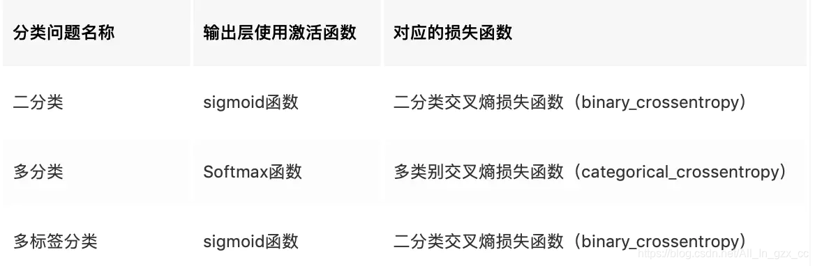
多标签的问题的损失函数是什么

这里需要先了解一下softmax 与 sigmoid函数，因为sigmoid函数一般和BCELoss，BCEWithLogitsLoss一起使用。softmax和CrossEntropyLoss一起使用

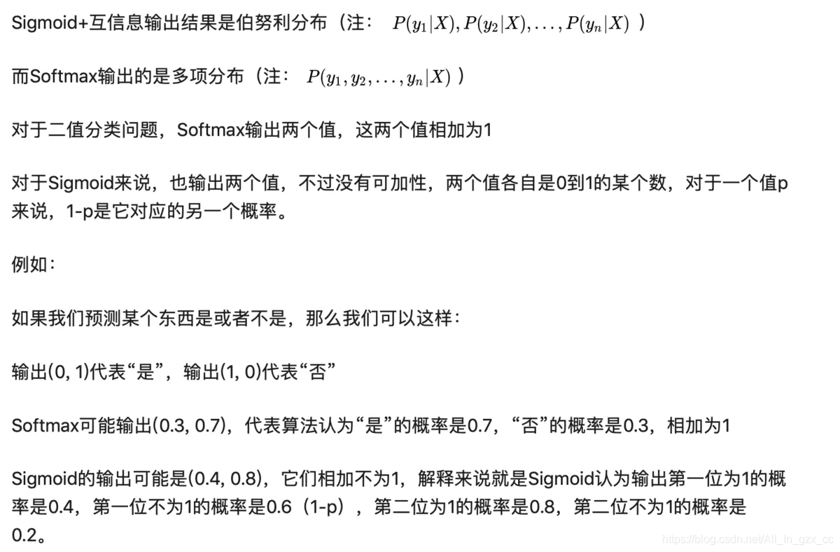
Sigmoid函数针对两点分布提出。神经网络的输出经过它的转换，可以将数值压缩到(0,1)之间，得到的结果可以理解成分类成目标类别的概率P，而不分类到该类别的概率是(1 - P)，这也是典型的两点分布的形式。Softmax函数本身针对多项分布提出，当类别数是2时，它退化为二项分布。而它和Sigmoid函数真正的区别就在——二项分布包含两个分类类别（姑且分别称为A和B），而两点分布其实是针对一个类别的概率分布，其对应的那个类别的分布直接由1-P得出。简单点理解就是，Sigmoid函数，我们可以当作成它是对一个类别的“建模”，将该类别建模完成，另一个相对的类别就直接通过1减去得到。而softmax函数，是对两个类别建模，同样的，得到两个类别的概率之和是1。

BCELoss

输入：（[B,C], [B,C]）,代表（prediction,target）的维度，其中，B是Batchsize，C为样本的class，即样本的类别数。

import torch
from torch import nn
 
input = torch.randn(3) # (3,1) 随机生成一个输入，没有被sigmoid。
print(input)
print(input.shape)
target=torch.Tensor([0., 1., 1.])
loss1=nn.BCELoss()
print("BCELoss:",loss1(torch.sigmoid(input), target))#需要sigmod
 
 
输出：
BCELoss: tensor(1.0053)

BCEWithLogitsLoss

输入：（[B,C], [B,C]）,输出：一个标量

import torch
from torch import nn
 
input = torch.randn(3) # (3,1) 随机生成一个输入，没有被sigmoid。
print(input)
print(input.shape)
target=torch.Tensor([0., 1., 1.])
loss2=nn.BCEWithLogitsLoss()
print("BCEWithLogitsLoss:",loss2(input,target))#不需要sigmoid
 
 
输出：
BCEWithLogitsLoss: tensor(1.0053)

CrossEntropyLoss

输入：（[B,C], [B]） 输出：一个标量（这个minibatch的mean/sum的loss）

nn.CrossEntropyLoss计算过程：

• input: logits(未经过softmax的模型的"输出”)
• softmax(input)
• -log(softmax(input))
• 用target做选择提取(关于logsoftmax)· mean

等价于：nn.CrossEntropyLoss = nn.NLLLoss(nn.LogSoftmax)

import torch
from torch import nn
 
loss2 = nn.CrossEntropyLoss(reduction="none")
target2 = torch.tensor([0, 1, 2])
predict2 = torch.tensor([[0.9, 0.2, 0.8], [0.5, 0.2, 0.4], [0.4, 0.2, 0.9]])
print(predict2.shape) # torch.Size([3, 3])
print(target2.shape) # torch.Size([3])
print(loss2(predict2, target2))
 
# #结果计算为：
# tensor([0.8761, 1.2729, 0.7434])

举例

1. BCEWithLogitsLoss计算ACC和Loss：

criterion = nn.BCEWithLogitsLoss()
# 计算准确率
def binary_accuracy(predicts, y):
    rounded_predicts = torch.round(torch.sigmoid(predicts))
    correct = (rounded_predicts == y).float()
    accuracy = correct.sum() / len(correct)
    return accuracy
 
 
# 训练
def train(model, iterator, optimizer, criterion):
    model.train()
    epoch_loss = 0
    epoch_accuracy = 0
    for batch in tqdm(iterator, desc=f'Epoch [{epoch + 1}/{EPOCHS}]', delay=0.1):
        optimizer.zero_grad()
        predictions = model(batch.text[0]).squeeze(1)
        loss = criterion(predictions, batch.label)
        accuracy = binary_accuracy(predictions, batch.label)
        loss.backward()
        optimizer.step()
        epoch_loss += loss.item()
        epoch_accuracy += accuracy.item()
    return epoch_loss / len(iterator), epoch_accuracy / len(iterator)

2. 计算ACC和Loss

# 截取情感分析部分代码 
    criterion = nn.CrossEntropyLoss()
    total_loss = 0.0
    correct_predictions = 0
    total_predictions = 0
   for batch in train_loader:
        input_ids = batch['input_ids'].to(device)
        labels = batch['label'].to(device)
 
        optimizer.zero_grad()
 
        logits = model(input_ids)
        loss_sentiment = criterion(logits, labels.long())
       
        loss_sentiment.backward()
        optimizer.step()
 
        total_loss += loss_sentiment.item()
 
        # get sentiment accuracy
        predicted_labels = torch.argmax(logits, dim=1)
        correct_predictions += torch.sum(predicted_labels == labels).item()
        total_predictions += labels.size(0)
 
    accuracy = correct_predictions / total_predictions
    loss = total_loss / len(train_loader)

总结

• 不管是二分类还是多分类，其实都可以只用CELOSS，只要target满足[0, 1, 2, …]
• BCELOSS和CELOSS的最大区别就是，BCE输出的是每个类的概率，而CE则约束了唯一类的概率。因此二/多分类可以无脑用CE，但是多标签更适合BCE