


背景
- hologres业务高峰期,大量来自CEM的任务容易造成OOM
- CEM无法识别sql复杂程度,执行时长不可控
- CEM没有sql调度中心,无法对sql查询任务进行动态管理
样本集
原始来源
来着于hologres的历史查询记录可以获得可用样本
- 只获取查询成功的SELECT语句
- 只获取开头为WITH的复杂查询,多为分析sql的临时表sql结构
- 只获取来自测试环境和生产环境的sql
SELECT
    COUNT(1) as count
FROM hologres.hg_query_log
WHERE
  command_tag='SELECT'
  AND status = 'SUCCESS'
  AND datname='ry_cdm_hl'
  AND client_addr in ('xx.xx.xx.xx','xx.xx.xx.xx')
  AND query like 'WITH%'
特征工程
由历史记录可以获得具体执行的sql以及执行时长,这本身就是样本对(sql–>duration)。由于执行时长(duration)是个数值,样本构造仅需要对sql语句进行处理
Explain
从explain <sql> 获取执行计划,解析执行计划顺序构造成二叉树,二叉树节点为执行计划节点的扫描函数。
执行计划是从下到上进行计算sql的,这里是hologres单节点执行sql的情况,构建出的二叉树是个极不平衡树(只会有左节点)。有些复杂sql可以构建出左右子树存在的平衡二叉树
Sort  (cost=0.00..31806.28 rows=926859 width=30)
  Sort Key: (CASE WHEN ("_$title" IS NULL) THEN 'NULL'::text ELSE "_$title" END), (FINAL pg_catalog.count((PARTIAL pg_catalog.count(1)))) DESC
  ->  Gather  (cost=0.00..555.17 rows=926859 width=30)
        ->  Final HashAggregate  (cost=0.00..487.63 rows=926859 width=30)
              Group Key: (CASE WHEN ("_$title" IS NULL) THEN 'NULL'::text ELSE "_$title" END), "_$event"
              ->  Redistribution  (cost=0.00..379.01 rows=5088503 width=30)
                    Hash Key: (CASE WHEN ("_$title" IS NULL) THEN 'NULL'::text ELSE "_$title" END), "_$event"
                    ->  Local Gather  (cost=0.00..355.12 rows=5088503 width=30)
                          ->  Decode  (cost=0.00..354.60 rows=5088503 width=30)
                                ->  Partial HashAggregate  (cost=0.00..354.50 rows=5088503 width=30)
                                      Group Key: (CASE WHEN ("_$title" IS NULL) THEN 'NULL'::text ELSE "_$title" END), "_$event"
                                      ->  Filter  (cost=0.00..205.43 rows=27936128 width=22)
                                            Filter: ((CASE WHEN ("_$title" IS NULL) THEN 'NULL'::text ELSE "_$title" END) <> ''::text)
                                            ->  Project  (cost=0.00..159.47 rows=27936128 width=22)
                                                  ->  Seq Scan on Partitioned Table dwd_log_cem_event_enet  (cost=0.00..127.74 rows=35277948 width=27)
                                                        Partitions selected: 7 out of 161
                                                        Filter: ((ds >= 20231115) AND (ds <= 20231121))
Optimizer: HQO version 2.0.0
Optimizer: HQO version 2.0.0
构造Tensor
一颗二叉树代表了sql的执行计划,也间接代表了sql的复杂程度(由执行计划的顺序和扫描行数共同决定)
对于二叉树–>Tensor,这边主要是由这棵树的前中后序遍历结果进行构造,因为前中后序遍历决定当且仅当的一棵树
普通特征矩阵
这边构造了两种Tensor,一种是普通特征矩阵[batch_size,500,3]
- 维度1(500):前中后序遍历的最大长度,目前所有sql的前中后序遍历加起来长度也就00出头,500的容量完全够用(遍历长度不足500,补0.0)
- 维度2(3):二叉树节点保存的rows、width以及算子名称。目前样本中sql执行计划出现过的算子最多20多个,直接映射成0-20+的数值即可(编码)
import re
from queue import LifoQueue

from sql_time_pred.holo.entity.history import History
from sql_time_pred.holo.entity.operator_node import OperatorNode


def refine_plan(plan):
    return [p for p in plan if "cost=" in p and "rows=" in p and "width=" in p]


def head_space_count(text):
    pattern = r'^\s+'
    # 使用正则表达式找到匹配项
    match = re.search(pattern, text)
    # 如果找到匹配项,则计算空格的数量
    if match:
        count_spaces = len(match.group())
    else:
        count_spaces = 0
    return count_spaces


def parse_plan(duration: int, plan: list[str]):
    # 去除无用信息
    plan = refine_plan(plan)
    root_line = plan[0]
    root = OperatorNode(root_line)
    root_space_count = head_space_count(root_line)
    root.level = root_space_count
    root.duration = duration

    stack = LifoQueue()
    indent_stack = LifoQueue()
    stack.put(root)
    indent_stack.put(root_space_count)

    for i in range(1, len(plan)):
        line = plan[i]
        space_count = head_space_count(line)
        node = OperatorNode(line)
        node.level = space_count
        node.duration = duration

        if space_count > indent_stack.queue[-1]:
            stack.queue[-1].left_node = node
            stack.put(node)
            indent_stack.put(space_count)
        else:
            while space_count <= indent_stack.queue[-1]:
                stack.get()
                indent_stack.get()
            stack.queue[-1].right_node = node
            stack.put(node)
            indent_stack.put(space_count)

    return root


def build_nodes(histories: list[History]) -> list[OperatorNode]:
    plans = [(his.duration, his.plan) for his in histories]
    return [parse_plan(duration, plan) for duration, plan in plans]


def validate_parse_nodes(histories: list[History]):
    nodes = build_nodes(histories)
    assert len(nodes) == len(histories)
    for i in range(len(histories)):
        plan0 = []
        print_node(nodes[i], plan0)
        plan = histories[i].plan
        plan = refine_plan(plan)
        print(plan == plan0)


def print_node(root: OperatorNode, plan: list[str]):
    if root == None:
        return
    plan.append(root.message)
    print_node(root.left_node, plan)
    print_node(root.right_node, plan)
Image(主要用于后续的CNN方案)
前中后序遍历也仅仅是用节点顺序表达一棵树,是否可以构造出更为直观保留树结构和节点信息的Tensor?
对一棵树的遍历映射成二维特征矩阵,前中后序遍历可以获得一个Image[batch_size,3,500,500]
- 维度1(3):前中后序遍历
- 维度2、3(500):容纳树的遍历最多用500*500的Tensor保存,同上,也是够用的
100, 0, 0,   0, 0,   0
200, 0, 200, 0, 0,   0
300, 0, 300, 0, 300, 0
文本编码
除去计算机语言特性,sql语句本身就是文本,完全可以用NLP的方式进行编码
import random
import re

import torch
from nltk.tokenize import word_tokenize

# 示例文本
text = '''
with temp_event_table as(
select
   case
      when cast(event_cem._$title as text) is null then 'NULL'
      else cast(event_cem._$title as text)
   end as group_cem,
   event_cem.ds as ds_cem,
   event_cem._$event as _$event_cem,
   event_cem._$time as _$time_cem,
   event_cem._$one_id as _$one_id_cem
from
   ry_cdm.test_dwd_log_cem_event_enet event_cem
where
   (event_cem.ds >= 20231111
      and event_cem.ds <= 20231124)
   and ((event_cem._$event = '$AppStart')
      or (event_cem._$event = '$AppEnd')) ),
temp_bool_table as(
select
   temp_event_table.group_cem,
   temp_event_table._$one_id_cem,
   DATE(TO_TIMESTAMP(temp_event_table._$time_cem / 1000)) as date_cem,
   case
      when temp_event_table._$time_cem >= 1699632000000
         and temp_event_table._$time_cem <= 1700236800000
         and (temp_event_table._$event_cem = '$AppStart') then true
         else false
      end as start_cem,
      case
         when temp_event_table._$time_cem >= 1699718400000
            and temp_event_table._$time_cem <= 1700841600000
            and (temp_event_table._$event_cem = '$AppEnd') then true
            else false
         end as end_cem
      from
         temp_event_table ),
temp_retention_table as(
select
   temp_bool_table.group_cem,
   temp_bool_table._$one_id_cem,
   RANGE_RETENTION_COUNT(temp_bool_table.start_cem,
   temp_bool_table.end_cem,
   temp_bool_table.date_cem,
   array[1,
   2,
   3,
   4,
   5,
   6,
   7],
   'day',
   'normal') as retained_detail_cem
from
   temp_bool_table
group by
   temp_bool_table.group_cem,
   temp_bool_table._$one_id_cem ),
temp_merge_table as(
select
   temp_retention_table.group_cem,
   temp_retention_table._$one_id_cem,
   REGEXP_SPLIT_TO_ARRAY(unnest(RANGE_RETENTION_SUM(temp_retention_table.retained_detail_cem)), ',')as retained_cem
from
   temp_retention_table
group by
   temp_retention_table.group_cem,
   temp_retention_table._$one_id_cem ),
temp_split_table as(
select
   temp_merge_table.group_cem,
   temp_merge_table._$one_id_cem,
   temp_merge_table.retained_cem[1] as first_day_cem,
   temp_merge_table.retained_cem[2] as init_people_cem,
   temp_merge_table.retained_cem[3] as retention_1_cem,
   temp_merge_table.retained_cem[4] as retention_2_cem,
   temp_merge_table.retained_cem[5] as retention_3_cem,
   temp_merge_table.retained_cem[6] as retention_4_cem,
   temp_merge_table.retained_cem[7] as retention_5_cem,
   temp_merge_table.retained_cem[8] as retention_6_cem,
   temp_merge_table.retained_cem[9] as retention_7_cem,
   temp_merge_table.retained_cem[10] as retention_8_cem,
   temp_merge_table.retained_cem[11] as retention_9_cem,
   temp_merge_table.retained_cem[12] as retention_10_cem,
   temp_merge_table.retained_cem[13] as retention_11_cem,
   temp_merge_table.retained_cem[14] as retention_12_cem,
   temp_merge_table.retained_cem[15] as retention_13_cem,
   temp_merge_table.retained_cem[16] as retention_14_cem,
   temp_merge_table.retained_cem[17] as retention_15_cem
from
   temp_merge_table )
select
   distinct temp_split_table._$one_id_cem as _$one_id,
   account_cem._$login_id,
   account_cem.account_id,
   account_cem.account_tenant_id,
   account_cem.account_company_id,
   account_cem.account_name,
   account_cem.account_phone_decrypt,
   account_cem.is_real_name_account,
   account_cem.account_identy_type,
   account_cem.account_l1_zone,
   account_cem.account_l2_zone,
   account_cem.account_nation,
   account_cem.account_provnce,
   account_cem.account_city,
   account_cem.account_first_visit_app_time,
   account_cem.account_first_visit_macc_time,
   account_cem.account_last_visit_app_time,
   account_cem.account_last_visit_macc_time,
   account_cem.use_duratn,
   account_cem.use_cnt,
   account_cem.account_type,
   account_cem.account_registr_date,
   account_cem.account_active_date,
   account_cem.account_repurce_date,
   account_cem.account_loyal_date,
   account_cem.account_valid_proj_cnt,
   account_cem.account_rui_proj_cnt,
   account_cem.account_yi_proj_cnt,
   account_cem.account_home_proj_cnt,
   account_cem.account_device_cnt,
   account_cem.account_rui_device_cnt,
   account_cem.account_yi_device_cnt,
   account_cem.account_home_device_cnt,
   account_cem.account_proj_sum_price,
   account_cem.account_ry_proj_sum_price,
   account_cem.account_first_rui_proj_online_date,
   account_cem.account_first_yi_proj_online_date,
   account_cem.account_certify_enginer_type,
   account_cem.account_company_name,
   account_cem.account_company_role_type,
   account_cem.company_owner_account_name,
   account_cem.company_class,
   account_cem.company_employe_cnt,
   account_cem.company_certify_enginer_cnt,
   account_cem.company_proj_cnt,
   account_cem.company_scheme_cnt,
   account_cem.company_device_cnt,
   account_cem.case_total_cnt,
   account_cem.case_cnt_rct_1m,
   account_cem.case_cnt_rct_6m,
   account_cem.case_cnt_rct_1y,
   account_cem._$carrier,
   account_cem._$manufacturer,
   account_cem._$model,
   account_cem._$browser,
   account_cem._$browser_version,
   account_cem._$os,
   account_cem._$os_version,
   account_cem._$screen_height,
   account_cem._$screen_width
from
   ry_ads.ads_log_cem_user_account_label_wt_enet account_cem
right join temp_split_table on
   temp_split_table._$one_id_cem = account_cem._$one_id
where
   temp_split_table.init_people_cem::INTEGER >= 1
   and temp_split_table.group_cem = ''
   and temp_split_table.first_day_cem = '20231111'
limit 15 offset 0
'''
device = torch.device("cuda" if torch.cuda.is_available() else "cpu")

text = re.sub(r'\s+', ' ', text)
# 分词
tokens = word_tokenize(text)

# 构建词汇表
vocab = sorted(list(set(tokens)))

# 随机打乱词汇表顺序
seed = 213422
random.seed(seed)
random.shuffle(vocab)

word_to_index = {word: i for i, word in enumerate(vocab)}

# 将文本转换为索引序列
indexed_tokens = [word_to_index[word] for word in tokens]

# 将索引序列转换为张量
tensor = torch.tensor(indexed_tokens)
tensor = tensor.to(device)

# 打印结果
print(tensor)
但这种编码方案十分依赖足量样本,以保证样本的泛化足够
举例:
这两句sql文本上就差了个数字2,文本编码出来的Tensor十分类似,但是两者执行复杂度天差地别。样本很少时,使用文本编码,会造成严重的样本倾斜
-- 简单sql,查询7天数据
SELECT * FROM ry_cdm.dwd_log_cem_event_enet
WHERE ds >= 20231115 and event_cem.ds <= 20231121
-- 复杂sql,查询一年数据
SELECT * FROM ry_cdm.dwd_log_cem_event_enet
WHERE ds >= 20221115 and event_cem.ds <= 20231121
样本倾斜
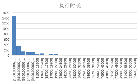
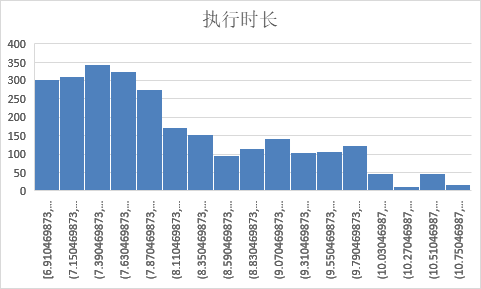
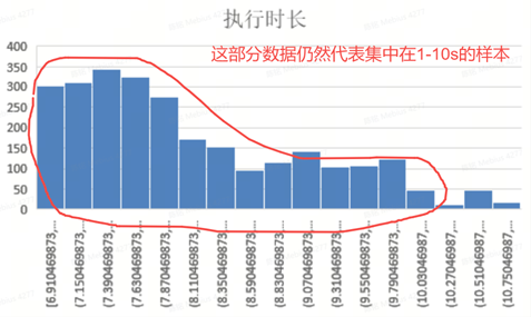
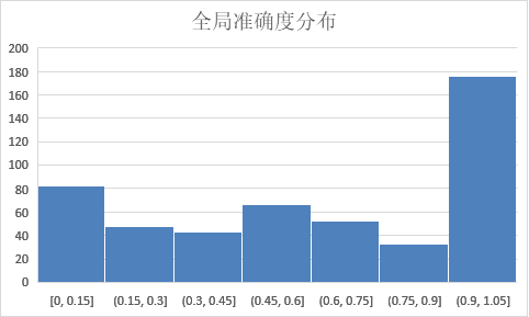
目前样本中的执行时长大部分集中在1s左右,这就造成大量样本对的输出基本就是1秒多,训练出来的模型由于样本倾斜,也只会输出1s左右的预测。
用log函数对其进行离散化
self.duration = [math.log(x + math.e, math.e) for x in self.duration]
离散化前的执行时长分布
离散化后的执行时长分布
标准化
主要针对sql转换成的Tensor进行标准化,执行计划中行数大的可达几百亿,小的只有个位数,标准化可以避免大数值影响梯度下降
def norm(self, tensor):
    tensor = torch.log(tensor + 1)  # 添加1以避免log(0)
    # 标准化(零均值,单位方差)
    mean = tensor.mean()
    std = tensor.std(dim=0) + 0.0001
    tensor = (tensor - mean) / std
    return mean, std, tensor
模型
特征矩阵欧式距离
原理
对现有样本的sql都构造成Image,即三维特征矩阵。任意的sql都可以构造Image,和样本的Image进行相似度比对。矩阵相似度计算方式有很多,这里用最小的欧氏距离获取样本中最相似的Image,进而获得对应样本的执行时长。
优点
- 模型不需要训练,不需要额外的GPU资源
- 易于实现,执行效率高
##¥ 缺点 - 精度差,受限于样本过少,即使匹配到最相似的样本,其欧氏距离仍旧很大,获得的执行时长并不准
CNN
原理
对于Image样本进行CNN分类任务。全连接层直接预测时长
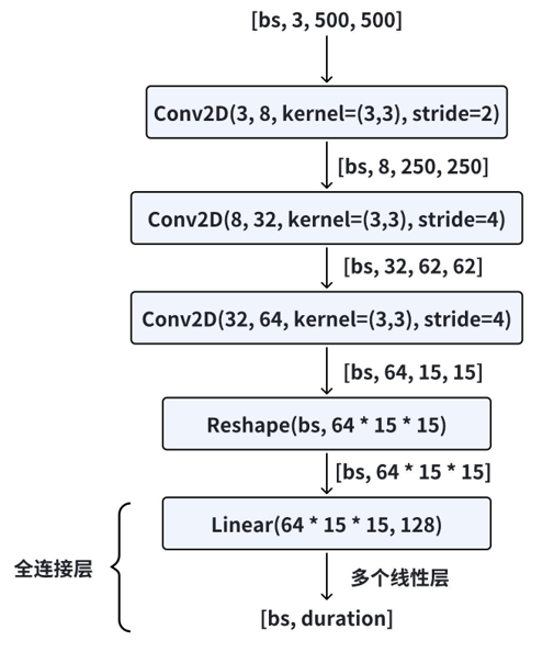
优点
- 实现简单,CNN会帮你处理好数据中的结构信息
缺点
- Image中存在大量0数据,数据过于稀疏,梯度下降困难
- 样本过少,预测时长不够准确
LSTM+ResNet3/5
这里的LSTM用了8层,输出的维度由原来3扩充为了32
import torch
from torch import nn
from torch.nn import functional

from sql_time_pred.dataset.sample_builder import max_seq_length, vector_size

use_res_net = True


class ResBlock(nn.Module):
    def __init__(self, ic, oc, class_num):
        super(ResBlock, self).__init__()

        self.ic = ic
        self.oc = oc
        self.class_num = class_num

        self.linear1 = nn.Linear(ic, oc)
        self.bn1 = nn.BatchNorm1d(class_num)

        self.linear2 = nn.Linear(oc, oc)
        self.bn2 = nn.BatchNorm1d(class_num)

        # 短接回路
        self.extra = nn.Sequential()
        if oc != ic:
            self.extra = nn.Sequential(
                nn.Linear(ic, oc),
                nn.BatchNorm1d(class_num)
            )

    def forward(self, x):
        # 计算残差块的卷积输出
        out = functional.relu(self.bn1(self.linear1(x)))
        out = self.bn2(self.linear2(out))

        # 计算短接的输出并相加
        out = self.extra(x) + out
        out = functional.relu(out)
        return out


class LSTM(nn.Module):

    def __init__(self, class_num: int,
                 hidden_size: int,
                 num_layers: int,
                 res_layer_num: int):
        super(LSTM, self).__init__()
        self.hidden_size = hidden_size
        self.class_num = class_num
        # [batchSize,max_seq_length,vectorSize] --> [batchSize,max_seq_length,hidden_size]
        self.lstm = nn.LSTM(
            input_size=vector_size,
            hidden_size=self.hidden_size,  # hidden_layer的数目,即输出的维度
            num_layers=num_layers,
            batch_first=True,  # 输入数据的维度一般是(batch, squence, vector),该属性表征batch是否放在第一个维度
        )
        self.seq = nn.Sequential(
            nn.Linear(int(max_seq_length * self.hidden_size / self.class_num), 1024), nn.ReLU(),
            nn.Linear(1024, 512), nn.ReLU(),
            nn.Linear(512, 128), nn.ReLU(),
            nn.Linear(128, 1), nn.ReLU(), )

        assert res_layer_num == 3 or res_layer_num == 5
        channels = [512, 256, 128, 64, 32][::int(3 - (res_layer_num - 1) / 2)]
        channels = [int(max_seq_length * self.hidden_size / self.class_num)] + channels
        self.res_seq = nn.Sequential()
        for i in range(len(channels) - 1):
            self.res_seq.add_module("res_net_" + str(i), ResBlock(channels[i], channels[i + 1], class_num))
            self.res_seq.add_module("relu_" + str(i), nn.ReLU(), )
        self.fc = nn.Sequential(
            nn.Linear(32, 16), nn.ReLU(),
            nn.Linear(16, 1), nn.ReLU(),
        )

    def forward(self, x):
        output, h_c = self.lstm(x)
        output = torch.reshape(output, (-1, self.class_num, int(output.shape[1] * output.shape[2] / self.class_num)))

        if use_res_net:
            output = self.res_seq(output)
        else:
            output = self.seq(output)
        output = self.fc(output)
        # [1,20,1]
        output = torch.reshape(output, (-1, self.class_num))
        # [1,20]
        return output


if __name__ == '__main__':
    l = [512, 256, 128, 64, 32][:1]
    device = torch.device("cuda" if torch.cuda.is_available() else "cpu")
    randn = torch.randn(1, 500, 3).to(device)
    net = LSTM(20).to(device)
    net1 = net(randn)
    print()
优点
- sql执行计划可以视作时序信息,本质上代表了hologres的运行顺序,由LSTM提取特征比较合适
- 精度最高,当然模型参数量也最多
- 全连接层由多层线性层转为了多个ResNet残差块
- 由原先的预测执行时长转为分类任务,在分类数比较多的时候,同样可以预测细粒度的时长
- 多中分类数量可以训练多个模型,做集成学习
缺点
- 系统复杂度提升,模型代码量较多
- 提升模型维护门槛
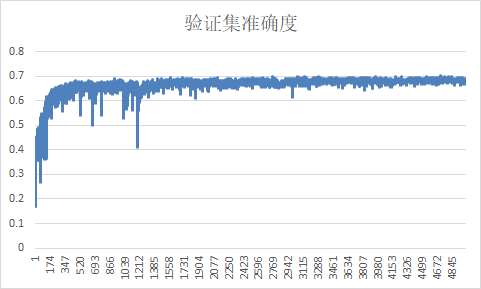
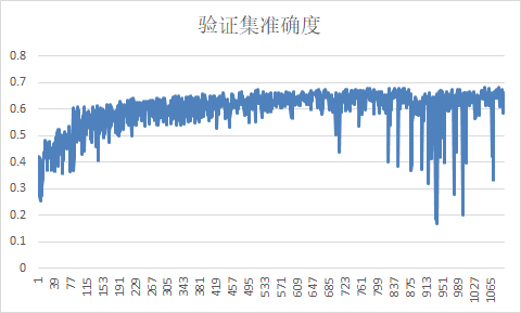
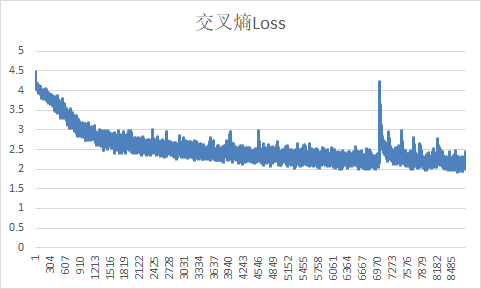
模型测试
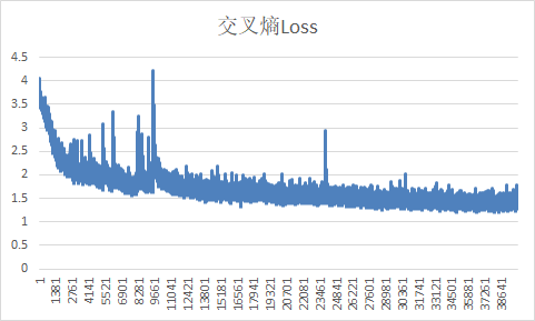
50分类
以训练5000轮的结果为例,训练参数如下
训练参数
[
    {
        "cls_weight":false,
        "res_layer_num":5,
        "hidden_size":32,
        "num_layers":5,
        "batch_size": 256,
        "epochs": 5000,
        "class_num": 50,
        "learn_ratio": 0.001
    }
]
训练基准
测试基准
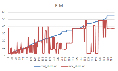
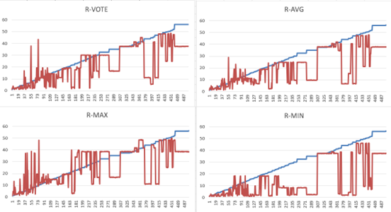
在0-10s内准确度在80%以上
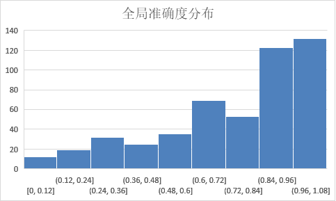
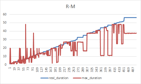
- R:真实的执行时长
- M:模型预测时长
样本离散化失效了?
并不是,交叉熵损失设置权重,仅仅是帮助训练时梯度下降的更快,尽量让模型学习稀疏部分的执行时长。
离散化也是在帮助梯度下降,样本倾斜的事实并没有改变,只是把集中在1-10s的样本离散在更大的数学空间上了。
样本质量决定了模型的上限,模型最好的性能也只能体现在了1-10s区间的预测了。
80分类
以训练1000轮的结果为例,训练参数如下
训练参数
[
    {
        "cls_weight":false,
        "res_layer_num":5,
        "hidden_size":32,
        "num_layers":5,
        "batch_size": 256,
        "epochs": 1000,
        "class_num": 80,
        "learn_ratio": 0.001
    }
]
训练基准
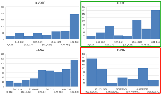
测试基准
在0-10s内准确度在70%以上
- R:真实的执行时长
- M:模型预测时长
集成学习
集成40、50、62、80分类的四个模型进行基准测试
改进了CEM什么?
队列系统,sql好好排队,合理打向数仓
现存问题
- 样本不足
- holo即将升配
评论区